Use Ranking System to Plan for Replacement
We are too focused on cost when it comes to thinking about equipment replacement. It certainly is important to know what it will cost to own and operate a unit in the year ahead and to make wise replacement decisions when the old unit—the defender—is likely to cost more than the minimum lifecycle cost you can expect from a new unit—the challenger. The defender-versus-challenger replacement theory is well accepted in practice, and many companies use this approach to plan replacements and manage fleet average age.
But there is more to it than cost. Other metrics such as age and utilization are important, and we frequently face the problem of balancing many factors when we try to identify or, at the very least, rank units for replacement.
The American Public Works Association (APWA) proposes the use of a simple subjective points system to rank vehicles for replacement. The system asks users to award a certain number of points for factors such as age, miles travelled, reliability, cost and condition, based on their assessment of each factor. The points are totaled, and the unit with the highest score “needs immediate consideration” for replacement. It has been proven to work, but it is subjective.
The need to combine many factors when trying to identify units for replacement is a common problem. Building on the APWA system, let’s add a little technology and develop a spreadsheet that combines subjectivity and analysis to give us a practical tool we can use to help in replacement decisions for large equipment groups such as pickups and tri-axle trucks.
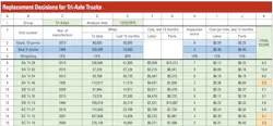
The nearby spreadsheet table serves as an example of how this might work with a grouping of tri-axle trucks.
Columns C, D, E, H, I and J show we are looking at six factors: year of manufacture; miles travelled, life to date; miles travelled in the past 12 months; a subjective inspection score; repair labor cost per mile; and repair parts cost per mile.
The unit numbers and the required data need to be entered into the green cells. Then calculate cost per mile for labor and parts by dividing columns F and G by column E to obtain the values in columns I and J.
To set up the scoring system, award “points” to each unit under each of the six factors. Determine what value is “good” and worthy of 10 points and what value is “unacceptable” and not worthy of any points. Rows 3 and 4 indicate those ranges. For example, a year of manufacture of 2013 or later is worth 10 points, and a year of manufacture of 1994 or earlier is worth zero. The process of deciding what is “good” and “bad” takes some discipline. You need to quantify your expectations for each factor and decide where the boundaries lie. It is not easy, but it is necessary. It makes the process repeatable, and once you have set the boundaries, the process is defendable.
Units will not be at the boundaries; some will be above expectations, some below expectations, and some in between. The next step is to decide how to apportion points regardless of where units fall. If they fall above and below the boundary, values are easy: 10 points or zero points. If they fall in between boundary values, we apportion the points on a straight-line basis defined by the values in rows 3 and 4.
The graph on the left shows how it is done for year of manufacture: zero points for units older than 1994, a straight-line proportion of the points between 1994 and 2013, and 10 points for units newer than 2013. The graph on the right shows how it is done for labor cost per mile travelled during the last 12 months: 10 points for under $0.09 per mile, a straight-line proportion between $0.09 and $0.30 per mile, and zero if the cost is more than $0.30 per mile.
These six factors do not, or should not, count equally in determining the final score. A weighting factor applied to each of the six factors aids in calculating the final score. In row 5, 30 percent of the weighting goes to factors that measure age (15 percent for age in years, column C, and 15 percent for age in miles, column D); 30 percent of the weight goes to utilization (miles in the last 12 months, column E); 30 percent of the weight goes to cost factors (cost per mile in the last 12 months for labor and parts, columns I and J); and 10 percent of the weight goes to the subjective inspection (column H).
With all the data in place, do the mathematics to determine the final score. It is a little technical but not complicated. The final score is the weighted total of the points calculated for each of the six factors considered.
Finally, use the analysis to help in your decisions. In this example, units in rows 9, 14 and 15 have low scores and are clearly candidates for replacement. Row 9 must go, the other two might depend on available capex budget. The unit in row 7 is better than the boundary values for all factors except labor cost per mile. It is a keeper, as are the units in rows 11, 8 and 6.
Tools like this enable us to move away from a fixation about cost. Other factors influence our decisions. We need to know how to include them.
