Equipment managers must take a long-term view of the repair/rebuild/replace decision in order to optimize the value of equipment assets over their full life cycle. They should not worry too much about short-term fluctuations; wise investments and wise decisions pay off. Not everyone sees it that way, unfortunately, and they often struggle with the curse of the annual budget when they know that longer-term, life cycle-based decisions produce better long-term results.
The Effects of Depreciation Policy
| 1 | 2 | 3 | 4 | 5 | 6 | 7 | 8 | 9 | 10 | 11 |
| Year | Hrs Worked | Dep Charges | Op Cost | Total | Revenue | Gain/Loss | Hrs Worked | O&O Cost | Revenue | Gain/Loss |
| 1 | 2000 | $20,000 | $10,000 | $30,000 | $40,000 | $10,000 | 2000 | $30,000 | $40,000 | $10,000 |
| 2 | 2000 | $20,000 | $15,000 | $35,000 | $40,000 | $5,000 | 4000 | $65,000 | $80,000 | $15,000 |
| 3 | 2000 | $20,000 | $20,000 | $40,000 | $40,000 | $0 | 6000 | $105,000 | $120,000 | $15,000 |
| 4 | 2000 | $20,000 | $25,000 | $45,000 | $40,000 | ($5,000) | 8000 | $150,000 | $160,000 | $10,000 |
| 5 | 2000 | $20,000 | $30,000 | $50,000 | $40,000 | ($10,000) | 10000 | $200,000 | $200,000 | $0 |
| 6 | 2000 | $35,000 | $35,000 | $40,000 | $5,000 | 12000 | $235,000 | $240,000 | $5,000 | |
| 7 | 2000 | $40,000 | $40,000 | $40,000 | $0 | 14000 | $275,000 | $280,000 | $5,000 | |
| 8 | 2000 | $45,000 | $45,000 | $40,000 | ($5,000) | 16000 | $320,000 | $320,000 | $0 | |
| 9 | 2000 | $50,000 | $50,000 | $40,000 | ($10,000) | 18000 | $370,000 | $360,000 | ($10,000) | |
| 10 | 2000 | $55,000 | $55,000 | $40,000 | ($15,000) | 20000 | $425,000 | $400,000 | ($25,000) | |
| Totals | 2000 | $325,000 | $425,000 | $400,000 | ($25,000) |
There is a clear distinction between annual costs and life cycle, or life-to-date, costs that will clear up a number of issues regarding depreciation and other transactions that occur on an annual basis. Lots of numbers are involved, so the simplified example in the table above will help in understanding the calculations.
The first thing to notice is that the calculation is divided into two parts. Columns 3 to 7 list the transactions that occur within each year and show what happens in each accounting or budget period. Columns 8 to 11 are life-to-date costs and revenues to give the picture over the full life cycle of the machine.
The second thing to notice is that the calculation shows both costs and revenue. This is done to illustrate how the difference between the estimated cost (column 5) and the estimated revenue (column 6) changes and to develop a “gain or loss” pattern for each year in the life of the machine (column 7).
Columns 1 and 2 show that we will keep the machine for 10 years and work 2,000 hours per year.
Column 3, depreciation charges, is where most of the controversy lies. The example machine has been purchased for $100,000, and the company has elected to allocate this cost over an assumed useful life of five years by charging depreciation at a uniform rate of $20,000 per year. This “depreciation policy” is critical to the calculation, as we’ll see later. For the purposes of this example, the depreciation charges in column 3 make up the owning costs of the machine. They could also be taken as the annual lease costs if the machine were leased rather than purchased.
Column 4 is the estimated operating cost for each year in the machine’s life, which increases as the machine ages. Column 5 totals columns 3 and 4 to give the total expected annual cost of the machine. Column 6 is the revenue that the machine can be expected to earn given an internal rental rate of $20 per hour.
Column 7 calculates the gain or loss expected from the machine in each year by subtracting column 5 from column 6. Notice how this changes over time. Years 1, 2 and 3 are “good” because the revenue is sufficient to cover the depreciation charges and the operating costs. Years 4 and 5 are “bad” because depreciation charges are still in play and operating costs have grown to the stage where annual revenue does not cover annual cost. Years 6 and 7 are “good” because depreciation charges have stopped and operating costs do not yet exceed revenue. Years 8, 9 and 10 are “bad” because operating costs exceed revenue. This good-bad swing is exactly the reason why a single-minded focus on annual results is such a dangerous thing.
Columns 8 to 11 show the life-to-date situation. Column 8 is hours worked, life to date. Columns 9 and 10 are the life-to-date accumulations of columns 5 and 6, respectively, and column 11 gives the life-to-date gain or loss on the machine by subtracting column 9 from column 10. This is the life-to-date or life cycle version of the up and down annual results given in column 7.
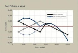
The graph below plots column 7 as the black line and column 11 as the dark blue line. The up and down nature of annual gains and losses is clear as is the fact that the assumed internal rental rate of $20 per hour used to calculate the revenue columns is sufficient to produce a $5,000 life-to-date gain at the economic or “sweet spot” life between 12,000 and 14,000 hours.
The depreciation policy plays an important role in the shape of both the black line and the blue line. Three things define the depreciation policy: the assumed useful life, the assumed residual value, and the portion of the total depreciation charged in each year. The policy used here (life = 5 years; residual value = 0 percent; total distributed = 20 percent per year) is not unusual. More conservative and risk-averse companies use a more aggressive policy (life = 4 years; residual value = 0 percent; total distributed = 40, 30 , 20 and 10 percent in successive years). Other companies are less conservative, or recognize that certain assets such as lattice-boom cranes have long lives and use flatter depreciation policies.
Two things are important with regard to the policy. First, the depreciation policy only affects the situation up to the time the asset is fully depreciated. After that, annual gains and losses are affected only by operating costs. Second, an aggressive policy may return the investment quickly and reduce financial risk, but it increases reluctance to make the investment because high early depreciation charges produce significant losses on revenue in early years.
This is shown in the graph where the gray line and the light blue line show the early negative results arising from changing the depreciation policy from that used in the example to a more aggressive policy where the full value is depreciated over four years at a rate of 40, 30, 20, and 10 percent in successive years. The graph also shows how the blue lines and the grey and black lines flow together once the machine has been fully depreciated and the policy no longer affects the situation.
We use fixed hourly internal rental rates to calculate the revenue earned by a machine, and we then analyze the difference between cost and revenue. Variations cause concern because we want steady results from month to month. But, as we have seen from the example, variations are frequently the result of the policy used to calculate depreciation charges. The policy needs to be consistent, conservative and in compliance with generally accepted accounting practice. It must also recognize that depreciation charges affect annual results and can easily put an inappropriate short-term focus on what should be wise, well-considered, long-term repair/rebuild/replace decisions.


