Most of us will agree that the hourly cost of a machine is strongly influenced by how much we use it and how long we keep it. Use it little or keep it for a short time, and cost per hour will be high because owning costs are high; keep it for a very long time, and cost per hour will be high because of all the money needed for repair parts and labor to keep the old unit working.
We will also agree that how long we keep the machine is strongly influenced by its hourly cost. No one, we hope, is going to keep a machine once its hourly owning and operating costs become systematically and progressively more expensive.
The strong relationship between cost and age is often overlooked, and most organizations focus almost entirely on cost management. They collect costs, calculate costs, and report costs but forget the simple fact that cost and age are two sides of the same coin. Much can be achieved and substantial savings are possible if organizations focus more on age and try to keep fleet average age at or around the elusive but critical “sweet spot,” where the sum of declining hourly owning cost and increasing hourly operating cost reaches a minimum.
Click here for more asset management.
The focus on cost rather than age probably comes from the belief that there is a single relatively fixed rate for a machine. The truth is that machines in a given category and class can have almost any “rate” depending on how long you keep them and how many hours you work them. The focus on a single rate is reinforced by the formats for the rate calculation found in most OEM performance handbooks. These start by requiring us to estimate an ownership period and an annual utilization and then use these estimates as the basis for the rest of the calculation. If the calculated rate comes to $73.00 per hour, nothing is done to emphasize the fact that this value is only valid if the machine is kept for an assumed ownership period of 8 years with a utilization of 1,750 hours per year. No calculations are done to find out if the assumed age and utilization produce a rate anywhere near the sweet spot, and it is silently assumed that the estimated ownership period and annual utilization are “optimum.”
A format based on single estimates for age and utilization is a hangover from the days when doing calculations and drawing graphs was slow and tedious. That is not the case anymore. There is no reason why the rate calculation should not be repeated many times based on many different values for age and utilization to determine both the magnitude and the timing of the sweet spot. The process is not complex. If we can do the calculation once based on an assumed age and utilization, then we can repeat it as often as necessary to determine the shape of the total owning and operating cost curve.
As with all rate calculations, the problem lies more in the assumptions we make than in the method we use to do the calculation. If we are going to do a sweet spot calculation, then we need two extra assumptions. First, we have to make some assumptions regarding the way in which residual market value changes with the age of the machine so that we can estimate different hourly owning costs for different ownership periods. This is not too complex; lots of auction data are available, and it is easy to make a reasonable estimate with reasonable accuracy. Next, we need to estimate the way in which the hourly cost of repair parts and labor increases as the machine ages. This is slightly more difficult, but (i) we know it is not constant with age, (ii) we spend a lot of time collecting historical data for units in our fleet, and (iii) if we can estimate repair parts and labor cost on the basis that we will keep the machine for a certain age, then we should be able to estimate it on the basis that we will keep the machine for shorter or longer periods.
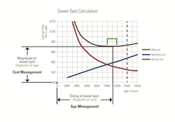
The diagram above shows the calculation done for an example machine. Owning costs, the green line, have been estimated at 2,000-hour intervals up to a maximum age of 16,000 hours. They come down steeply in the beginning and flatten toward the end based on the fact that the difference between the purchase price and the residual market value is spread over an increasing number of working hours. Operating costs, the blue line, have been calculated for the same period. They slope steadily upward based on an analysis of data that shows the life-to-date operating cost of a 6,000-hour machine is a little over $20 per hour while the life-to-date operating cost for a 14,000-hour machine is a little below $50 per hour.
Calculate total cost of ownership
The total owning and operating cost is given by the red line, which makes a minimum of $70 per hour at 11,000 hours. The sweet spot lies between 10,000 and 12,000 hours. It is not an exact science, and nothing is achieved by pretending to be more precise. A lot is achieved, however, by setting the target hours for the machine below the 14,000 hours (8 years at 1,750 hours per year) assumed in the original $73 per hour calculation (the dotted line).
Two questions are critical; “Why should I do it?” and “Is it worth it?” The answer is simply “Yes, you cannot manage cost without managing age.”
We are familiar with the process of using the hourly rate to establish cost management baselines. In our example, we would use the magnitude of the sweet spot to set a rate of $70 per hour and split this into two clear and distinct budgets: $31 per hour for all owning costs, and $39 per hour for all the operating costs. We would use these to generate revenue for the machine against which we offset actual costs in the normal way. We would be confident in our process knowing that we have tested our calculation over a range of ownership periods and annual utilization to determine the best balance between age and cost.
We are less familiar with the process of using the timing of the sweet spot to manage the average age of our fleet. At the moment, we probably do it by intuition and, at the moment, we probably do it fairly well. The problem with intuition is that it tends to yield funny results when we are pushed outside our comfort zone and beyond the limits of our experience. Many organizations are stretching the average age of their fleets and exploring new frontiers when it comes to equipment life. They are also trying to lower costs and reduce rates. It seems like, and it is, a tall order. Knowing the shape of the sweet spot curve and doing the rate calculation in a way that tells us what happens when we increase or decrease expected life is critical for success. We can no longer manage our fleet according to one benchmark—“The Rate.” We need to do the sweet spot calculation to establish three critical and strongly interrelated benchmarks:
- An owning cost rate against which we offset all the largely fixed costs of ownership.
- An operating cost rate against which we offset the hourly costs of running, maintaining and repairing our fleet.
- A target life to tell us when we lose the balance between age and cost, and when we start a time when each successive hour costs more than all the hours in the past.


