An equipment executive expects compliments for looking after the company’s assets. They expect longer lives and lower costs. But the real reason time and money are spent on maintenance is to stop machines from breaking down, disrupting operations, and changing carefully laid plans. We use equipment to produce work. Good machines help and support production while bad machines disrupt and delay production. We maintain machines because we want to stop them from breaking.
This approach simplifies discussion on availability and reliability. To measure availability, you need to measure the duration of downtime. To measure reliability, you simply need to record the fact that a down event took place. Availability has to do with the severity of downtime; reliability has to do with the frequency of down events.
Recording the fact that a down event occurred is binary: Did the machine or did the machine not go down and disrupt or delay production? You do not have to become involved with questions such as when it occurred, when it was reported, when the machine was returned to service, and when the machine actually recommenced work. You record the event by clearly and unambiguously coding time cards or work orders in a way that identifies reported emergency down events (RED events) as a specific and high-profile type of work, and then you specifically log and count each and every RED event.
The nearby table shows how only a little data is needed to do some interesting analysis. The numbers are factored data from a real machine. The values may not be real, but the lessons certainly are. Let’s go through the table and produce some charts to see what we can learn.
Columns A and B are all the data you need. Column A gives the hours worked life to date (LTD) when a work order arising from a RED event was completed. Column B gives the total cost of parts and labor on the work order. This is not a lot of data; it simply requires that RED events be coded as such and that hours worked LTD and costs are recorded.
Column C gives a count of RED work orders through the life of the machine. Row 9 shows that there were eight red events in the first 2,000 hours. Column D is the time between successive RED events. Row 5 shows that it was 300 hours between RED event #3 at 947 hours and RED event #4 at 1,247 hours. Column E is the mean time between failures life to date (MTBF LTD) calculated as column A divided by column C. Row 9 shows there were a total of eight RED events in the 2,000 hours to give an MTBF LTD of 250 hours.
Columns F and G are a little controversial. Some believe that rare events—such as RED work orders—should be measured in terms of the interval between events as has been done in columns D and E. Others believe that they should be measured in terms of a frequency or number of events in a given period as has been done in columns F and G. The conversion is simple: The interval of 300 hours in cell D5 converts to a frequency of 3.3 events per 1,000 hours in cell F5. The MTBF LTD of 250 hours in cell E9 converts to a frequency of 4.0 events per 1,000 hours LTD in cell G9.
Column H is the cumulative work order cost LTD, which is the running total of column B.
The table shows only the first 2,000 hours in the life of the machine. The full table runs for a total of 6,533 hours by which time the machine had accumulated 30 RED events for an MTBF LTD of 218 hours or an LTD frequency of 4.6 down events per 1,000 hours.
Two graphs present some analysis.
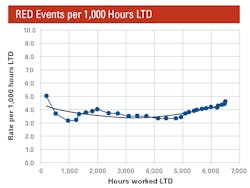
The first graph plots column G for the full data set.
It is a classic curve; failure frequency starts fairly high at the beginning while the machine works through some teething troubles. It then settles down to a rate of about 3.5 failures per 1,000 hours before starting to grow fairly aggressively around 4,500 hours. It is a classic bathtub wear out failure situation common to almost all construction equipment.
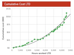
The second graph plots column H.
It is also a classic as we see repair parts and labor costs LTD rising exponentially as the machine ages. This is again common to almost all construction equipment and certainly common to most machines that experience wear out failure. As failure rates go up, costs go up.
Although the numbers are factored, the lessons are real. Notice that the failure rate starts to grow aggressively around 4,500 hours, and costs start to grow aggressively around 5,500 hours.
Can it be that failure rates are a lead indicator for cost growth? Failure rates must go up; then, and only then, will we spend on repair parts and labor.
We spend on maintenance because we want to stop our machines from breaking. We do this because high failure rates lead to high repair parts and labor costs.
Stop your machines from breaking.
Click here for more asset management.


