A great vintage takes time to mature. But when it does, it is marvelous. The same is true for a great idea. It takes time to go from the original concept to a practical valuable implementation.
We all know that old machines cost a lot in terms of the repair parts and labor needed to keep them running, reliable, and available. The H.B. Zachry Co. in San Antonio, Texas, operated an engineering services department with an equipment committee in the late 1950s and worked closely with Wm. K. Holt Machinery, its Caterpillar dealer, to do groundbreaking work that showed how repair expenditures increased with age. This gave rise to a 1968 Caterpillar publication, “The Fundamentals of Earthmoving,” that stated that “the repair costs for a single machine normally follow an upward stairstep pattern since major outlays for repairs usually come in spurts” and that “when averages are considered, the stairstep becomes a smooth upward curve.”
This article is dedicated to Zane Mitchell, who passed away in April.
Neither of these studies benefited from the rigorous statistical analysis techniques that became available in the 1990s. We had to wait until 1998 when Zane Mitchell analyzed field data from several companies to do groundbreaking research and develop a simple methodology for expressing the relationship between repair costs and age.
Zane’s research has matured. Many companies are using it to understand and analyze the optimum ownership period calculation, the sweet spot. Very smart people are working to implement Zane’s methods, and a few are now using it to quantify the replacement decision.
Read also: The Sweet Spot Revisited
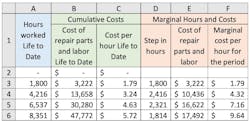
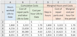
The calculations needed to quantify the replacement decision are not complicated, but two things are absolutely necessary. First, you need to know the life-to-date cumulative cost of repair parts and labor at various points in the life of the machine. There is nothing special about this; it is the same data that is required for any type of operating cost analysis at a unit level and is shown in columns A and B of the table at the top of this article.
Second, you need to have a clear understanding of the difference between cumulative costs and marginal cost. This is also illustrated in the table (left). The data gives us columns A and B: the hours worked by the machine, life to date (Column A), and the corresponding cumulative cost of repair parts and labor that point (Column B). The critical number, cumulative cost per hour, life to date is given in column C (B divided by A).
All the research quoted above and many years of field experience confirm that column B grows exponentially as the machine ages. Column C will therefore also grow over time to reflect the fact that the hourly cost of repair parts and labor increases as the machine ages; it becomes increasingly more expensive to keep running, reliable, and available.
Marginal cost—the cost of running the machine for one more period in the future—is of particular interest in the replacement decision as the past (life to date) is behind us and we are looking forward to decide what must be done in the future.
After you've read Mike's article, test your knowledge below.
Marginal costs are given in columns D, E, and F of the table. Column D is the step in the hours worked between two successive rows of data. For example, cell D4 represents the increase in hours between cell A4 (4,216 hours) and cell A3 (1,800 hours) and so on. Column E, the marginal cost of repair parts and labor for a given period, is the step in the cumulative cost column. For example, cell B4 minus cell 3B provides the value in E4. Column F, the marginal cost per hour for a given period, is column E divided by column D. This is the critical number: the estimated cost of repair parts and labor for that period in the life of the machine.
Read also: Extending the sweet spot on machine life
The fact that “major outlays for repairs usually come in spurts” means that the values in column F can swing quite a bit. There is, however, no doubt that they “follow a smooth upward curve” when “averages are considered” for a group of similar machines over a reasonable period.
The growth in the estimated marginal repair parts and labor cost per hour is a major factor in the replacement decision. Yes, age is important. Yes, we have used it a lot to define the optimum ownership period (sweet spot) and identify units that must be replaced. It is, however, a proxy for cost; age alone is of little help when it comes to quantifying the replacement decision and estimating the savings in repair parts and labor that can be achieved when units in a given group are replaced in a timely manner.
The second table (below) shows what happens to marginal cost per hour as an example group of haul trucks becomes progressively older. It follows the format used for the well-known “Churn Chart.” Let’s work through it and see what it tells us.
Rows 5 to 11 of columns A to F give the number, make, model, expected life, annual usage, and current age of the seven haul trucks in the group.
Rows 5 to 11 of columns G to K give the estimated marginal cost of repair parts and labor per hour for each machine in the next five years. The calculations were done in the same way as Column F in the first table, and we can see that the values grow year by year as each unit in the group ages.
The cells are color coded relative to a target value of $15 per hour using the scale shown in Row 2 – blue is for values less than $10 per hour, green for values between $10 and $15, yellow for values between $15 and $20, orange for values between $20 and $30, and red for values over $30 per hour.
The averages for the seven trucks in the rate group is given in row 12, columns G to K, which are also color coded.
We see that the average cost of repair parts and labor for the group is likely to be close to the target value of $15 in the next year, but the situation worsens steadily as the years progress and the units age. The growth in cost per hour is clearly driven by units MHT 14-1 and MHT 14-2, which are in the orange zone now and heading for the red zone. The hourly rate for these two units is well above target now and is likely to grow to twice the target rate in the next few years. Clearly these units are targets for replacement.
The total expected annual usage for the whole group of trucks is 12,800 hours (sum of E5 to E11). It is easy to multiply this by the average cost per hour for the group given in row 12 to obtain a good estimate for the total cost of repair parts and labor in each of the years ahead. The calculation shows that you can expect to spend about $184,000 on repair parts and labor in the next year (12,800 times $14.41) and about $300,000 in five years’ time (12,800 times $23.18). At this point, the average rate per hour for parts and labor for the whole group will be 25% above the target value ($18.79 divided by $15.00). The situation will only worsen if nothing is done.
Quantifying the savings in repair parts and labor expenditure that can be expected by replacing MHT 14-1 and MHT 14-2 is relatively simple. Simply delete MHT 14-1 and MHT 14-2 from the table and replace them with two new zero hour units. These will have low repair parts and labor rates in years 1 and 2 of their lives and then have marginal rates that are a lot like MTH 19-1 and MTH 19-2 by the time they reach about 6,000 hours of usage.
This has been done in the third table (below).
The first thing to notice is the absence of red cells. The whole picture is much better, and the average rate for the group is now $12.72 or 85% of target. Row 12 is as it should be, and there is no need to contemplate increasing the repair parts and labor portion of the internal charge out rate.
Redoing the estimated repair parts and labor expenditure calculation for the group using the new average rates shows that you can expect to spend about $104,000 on repair parts and labor in the next year (12,800 times $8.13) and about $221,000 in five years’ time (12,800 times $17.32).
Repeating this calculation for each year shows that the savings in repair parts and labor arising from the replacement of MHT 19-1 and MHT 19-2 comes to a little under $80,000 per year with a total of nearly $400,000 over the next five years.
So, if we replace the two oldest units now, we will save about $400,000 in repair parts and labor cost over the next five years. We will improve reliability, availability, and profitability, and we have at least $400,000 to put toward the owning cost of the two new units.
Quantifying the replacement decision and putting a number on the savings that can be achieved by replacing older units on time is a huge step forward. Yes, replacement can be delayed, but it cannot be denied. Delaying replacement impacts operating costs, reduces productivity, and lowers profits. It does, in the end, lead to a situation where the company cannot generate the financial resources needed maintain a viable productive fleet. This is the start of a downward spiral that few are able to survive.
Companies that learn and change are moving forward and achieving great results relative to those who simply want to defend the old way of doing things. Early work by Zachry and Holt gave us the concepts. The statistical analysis done by Zane Mitchell gave us the tools. Time has matured the process. It is time to enjoy the results.
About the Author

Mike Vorster
Mike Vorster is the David H. Burrows Professor Emeritus of Construction Engineering at Virginia Tech and is the author of “Construction Equipment Economics,” a handbook on the management of construction equipment fleets. Mike serves as a consultant in the area of fleet management and organizational development, and his column has been recognized for editorial excellence by the American Society of Business Publication Editors.
Read Mike’s asset management articles.


